If you are reading this, you probably know that machine learning has become one of the most vibrant and fast-growing research fields in computer science. Many of you might be familiar with terms like deep learning, convolutional neural networks and recurrent neural networks, or at least have come across them at some point. I mean, even mainstream magazines like Fortune and Forbes have featured articles on this subject, and last year Google Deepmind’s AlphaGo was all over the media.
It seems to me, though, that machine learning hasn’t gone mainstream within the software engineering community just yet. Maybe it’s because the mathematical aspect of it might seem scary and unappealing for a lot of software developers. Or maybe it’s just because it has only recently been that the world has gone crazy about artificial intelligence and we need more time to create better learning resources, adapted to audiences that don’t necessarily want to understand all the technical details.
In any case, I believe that the world would greatly benefit from having more developers interested in the field. Whereas researchers are more concerned about creating new and better techniques, machine learning practitioners would focus on applying them to solve real-world problems. I think that there are a number of tasks that could easily be solved using current machine learning techniques, but researchers don’t pay much attention to them simply because they are “too easy”.
In my first blog entry, I wanted to write a hands-on tutorial explaining one of these tasks and how I solved it. At the same time, I wanted to make the content of the tutorial accessible for anyone with minimum programming skills (even though the code is written in Python, it should be easy enough to follow for people familiar with other languages). You might be thinking that there are already dozens of beginner’s tutorials that explain how to classify handwritten digits using neural networks, and that’s exactly the reason why I wanted to do something different. Deep learning algorithms can be used to solve pretty much any task that involves making predictions, so why not start with something more interesting than a “Hello World”?
One of the often-heard difficulties of deep learning algorithms is that they need to be trained on very large datasets to work effectively. Although this is true, in many cases the data is easy to obtain or it can be generated by ourselves. At the end of this post, you will (hopefully) know how to train a convolutional neural network on data generated on-the-fly to predict the rotation angle needed to correct the orientation of a picture. This idea comes from a project that I started during the Deep Learning for Computer Vision summer seminar at UPC TelecomBCN in 2016. I have recently extended it and made it available on my GitHub page.
The first section of this post is a very short and basic introduction to neural networks so that everyone can follow the tutorial. Feel free to skip it if you are already familiar with the subject.
Short Introduction to Neural Networks
Artificial neural networks are machine learning algorithms vaguely inspired by biological neural networks. Different (artificial) neural network architectures are used to solve different tasks. Convolutional and recurrent neural networks are two of the most successful ones and they are largely responsible for the recent revolution of artificial intelligence. Convolutional neural networks (CNNs) are good at processing data that can be spatially arranged (2D or 3D). Typical use cases of CNNs are object detection and recognition. On the other hand, recurrent neural networks (RNNs) are good at processing sequences. They can be used to solve problems like speech recognition or machine translation. There are many different tasks that CNNs and RNNs can successfully solve, the only limit is your own imagination!
Neural networks are organised into interconnected layers of artificial neurons. Simply put, each layer takes the output of the preceding layer, applies a number of transformations, and sends its output to the next layer. The first layer’s input is connected to the raw data that we want to process (images, text, etc.) and the last layer output is whatever we want to predict.
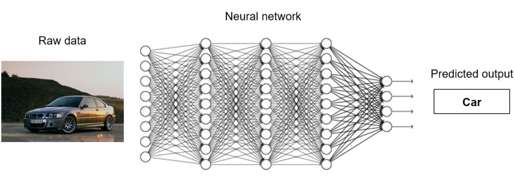
The purpose of the transformations that take place at each layer is to compute features. In machine learning, features are attributes that simplify the representation of the data. For example, if we are comparing two images, it’s easier to compare features that represent the texture at several points in the images than comparing the pixels one by one. Whereas in traditional machine learning algorithms these features needed to be carefully engineered by humans, a neural network learns how to compute the optimal features for the task at hand. Each layer in a neural network builds up on the features computed in the preceding layer to learn higher-level features. For example, in the neural network shown above, the first layer might compute low-level features such as edges, whereas the last layer might compute high-level features such as the presence of wheels in the image. In general, neural networks with more layers can learn higher-level features given that they are trained with more data, and because of this, they are said to have a better learning capacity. Neural networks with many layers are called deep neural networks. This is the reason why these kinds of machine learning algorithms are commonly known as deep learning.
Each connection in a neural network has a corresponding numerical weight associated with it. These weights are the neural network’s internal state. They are responsible for the different features that are computed at each layer. For a neural network (or any machine learning algorithm) to work, it needs to be trained. At the beginning of the training process, the weights are randomly initialized, so the network makes random predictions. During training, the network is fed with large amounts of labelled data and uses the prediction error (the error between the predicted output and the true output) to update its weights. Whenever the network makes a wrong prediction, the prediction error will be large. This will make the weights to be updated proportionally to that error so that the next time the network is fed with the same training sample, the prediction error will be lower. In other words, as the training progresses, the weights are updated to produce better features which help the network make better predictions. After many training iterations, the prediction error will be so low that the weights won’t be updated a significant amount. At that point, we can consider the training process finished. The function that computes the prediction error is typically called loss function, and the algorithm used to calculate the update of each weight during training is called backpropagation. Once the network is trained, the weights are fixed and the network can be used to predict unseen data.
Neural networks are usually trained on batches. Each time a batch is fed to the network, the prediction error is averaged over the whole batch using the loss function, and the network updates its weights based on that error. The reason to train using batches is simple. If the network is trained with only one sample at a time, the weight updates will be very inaccurate because the network will be optimising them based on individual samples. On the other hand, if the network is fed with the whole training set, the weight updates will be very accurate because they will be based on the average prediction error of all the training samples. In this case, though, the network will train very slowly because it can only update its weights once the whole training set has been fed. Using batches for training is a good trade-off: the noisy updates of training with individual samples are avoided, and the training process is quicker than if the whole training set was used because the weights are updated more frequently. Typical values for the batch size are 64, 128, 256 or 512.
During training, it is important to monitor the performance of the network on a subset of data that is not used for training. This is because machine learning algorithms tend to perform better on the data they have been trained on. By periodically testing on unseen data, we can ensure that the network generalises well to data outside of the training set. The subset of data used for this is typically known as the validation set.
Finally, let’s summarise the three most important types of layers that we will see in this tutorial:
Fully-connected layer: this is the simplest type of layer. It connects all its inputs to all the outputs of the preceding layer.
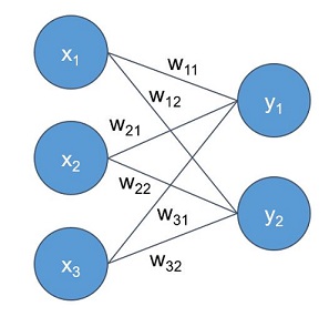
The output of each neuron is simply a weighted sum of its inputs. Considering the image above, representing this type of layer, the output of each neuron is as follows:
If you are familiar with calculus, you might notice how the above operations are equivalent to the mathematical dot product:
Convolutional layer: this is the type of layer that performs most of the computation in a convolutional neural network, hence their name. In essence, convolutional layers operate in a similar way to fully-connected layers. The difference is that the neurons are small kernels only connected to a small portion of the inputs, as opposed to all of them.
If you know image processing, you are probably familiar with convolutional kernels. These kernels are small two-dimensional windows that are slid over all the spatial locations in an image in order to compute a specific feature. This Wikipedia article shows several examples of typical convolutional kernels used in image processing and the features they compute. In neural networks, however, the kernels’ weights are not predefined, they are automatically learnt by the network during training. Moreover, CNNs use three-dimensional kernels, as they can operate over an arbitrary number channels. Deep convolutional neural networks typically use thousands of these kernels to compute different features.
Pooling layer: this type of layer downsample its input. Similar to convolutional layers, pooling layers consist of small sliding kernels that simply average spatial regions (average pooling) or take the maximum value (max pooling). Downsampling is typically used in convolutional neural networks to reduce the number of weights in consecutive layers, which in turn reduces their computational complexity. Pooling layers are not trainable since they don’t have any weights.
Some layers are usually followed by activation functions. These functions are applied to each neuron in the layers to decide whether they are active or not (a neuron is active if its output is greater than zero). They are in charge of providing the network with a non-linear behaviour.
And with that, we finish the introduction to neural networks. It was a lot of information in very few words, but I hope that at least you’ve got some of the key ideas. If you feel dizzy or didn’t quite understand something, don’t worry. Everything will be clearer once we start with the coding. And if you want to learn more about any of these topics, I have compiled a number of resources that have helped me to do so at the end of this post.
Problem Description
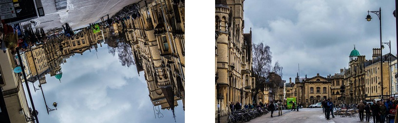
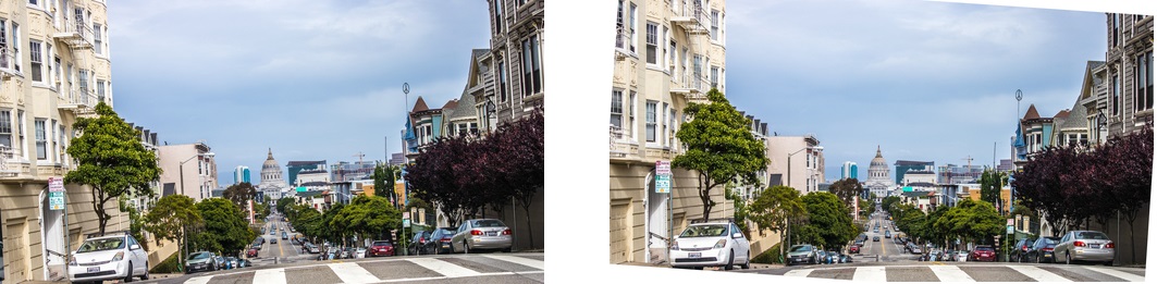
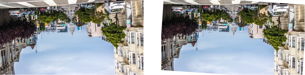
One of the things that I miss when I am looking at pictures or editing them is an option to automatically correct their orientation. Some software tools have the capability to straighten them, provided that the image is already in the right orientation. To illustrate that, let’s take a look at the Level tool of Adobe Photoshop Lightroom. As you can see in the images below, this kind of tool can correct small rotations with high accuracy (look at the edge of the road as a reference for the horizon).
But what happens if the image is upside down? As you can imagine, similar to the previous case, the corrected image is simply a straight version of the original.
Tools like this make use of image processing techniques to look for horizontal edges in the image and use them to rotate it in such a way that those edges are completely aligned with the horizon after the correction.
But what if we want the upside-down image to look like the original one? In order to do that we need an algorithm that can interpret the content of the image and act accordingly. In the previous case, we would easily figure out that the image is upside down by acknowledging the position of the sky and the road. That itself would be easy to do using image processing. But what if there is no sky or road in the image, or what if the content of the image is something completely different, like a person? It would be extremely difficult to write an algorithm that can take into account all the possible scenarios.
As you can image, this is the type of task that deep learning algorithms excel at. As you will see in the remainder of this post, this problem can be easily solved using a convolutional neural network.
Predicting Rotation Angle with Keras
In order to solve this task, we need to pick one of the many deep learning frameworks available. Nowadays Google’s TensorFlow seems to be becoming the industry standard; however, TensorFlow is somewhat low level and it can be a bit verbose, especially when it comes to defining deep neural networks. If you write raw TensorFlow code, you will probably end up writing a lot of helper functions to compose your models. Instead, a popular option is to use one of the many available libraries that wrap TensorFlow’s low-level functionality into high-level reusable functions. Everyone has their favourite. Google itself has added two of them to TensorFlow’s contrib module (TF Learn and TF-Slim) and another one to their main GitHub repository (PrettyTensor).
My favourite is Keras, although I have to say I haven’t tried all of them. Keras is built entirely with TensorFlow under the hood, so you can use it even if you are not familiar with it. You can also use it with Theano, another popular deep learning framework, as a backend. As you will see in the code snippets below, Keras code is very easy to write and extend thanks to its simple and modular design.
Preparing the data
The first thing we are going to do is to prepare the data. When preparing data for deep learning applications, we need to think about the format of the input data and the format of the output data (the labels). In our case, the format of the input data is clear: we want the network to process images. The output seems to be clear too. We need the network to predict the image’s rotation angle, which can then be used to rotate the image in the opposite direction to correct its orientation.
However, the output can be formatted in two different ways. One option is to predict a single value between 0 and 359 (or between 0 and 1 if normalised). This type of task is called regression. In this case, the label is simply the true value representing the rotation angle. In a regression task, the loss function could simply be the absolute difference between the predicted value and the true value, also known as the mean absolute error (MAE). For example, if our network sees an image rotated 10 degrees, but the predicted angle is 350 degrees, the MAE would be 340, right? Well, yes. But does this make sense to you? The angle difference between 10 and 350 degrees is actually exactly the same than between 10 and 30 degrees, i.e., 20 degrees. So the MAE is not a very good option because we would be calculating different prediction errors when in reality the angle difference is the same in both cases. This could easily be solved using a loss function that correctly computes the minimum difference between two angles.
The second option is to predict a class label. This type of task is called classification. If we want to treat our problem as a classification one, the network should produce a vector of 360 values instead of a single value. Each value of that vector represents the probability between 0 and 1 of each class being the correct one. The first entry of the vector would correspond to 0 degrees, the second entry to 1 degree, and so on. In this case, the label is a binary vector that contains 1 only in the entry that accounts for the true value. For example, if the network sees an image rotated 40 degrees, the output should ideally be a vector containing 0 (0% probability) at each entry except 1 (100% probability) in the 40th entry in order to match the label.
In my experiments, the network trained as a classifier worked much better than the regression one, so the rest of the tutorial will assume that we are solving a classification problem. I have uploaded both versions to the project’s GitHub repository, in case you are curious about the regression implementation. The large difference between these two is interesting in itself and might be a topic for a future post.
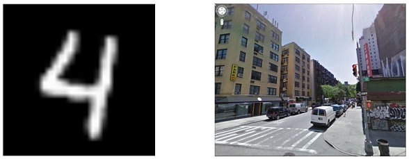
So now we know the format of our data, but how do we get it? Luckily, for this particular application, we can easily generate it ourselves. We simply need images with an orientation angle as close to 0 degrees as possible. In this way, we can rotate the images on-the-fly and take the rotation angles as the labels. I have done experiments with two different datasets: the MNIST database of handwritten digits (we are not going to classify them, I promise!) and the Google Street View dataset.
Keras makes it very easy to write data generators by extending one of the provided classes. In the code below you can see a basic implementation of a data generator that takes a NumPy array of input images and produces batches of rotated images and their respective rotation angles on-the-fly. This generator can also preprocess the input images if needed.
class RotNetDataGenerator(Iterator):

    def __init__(self, input, batch_size=64,
                 preprocess_func=None, shuffle=False):

        self.images = input
        self.batch_size = batch_size
        self.input_shape = self.images.shape[1:]
        self.preprocess_func = preprocess_func
        self.shuffle = shuffle
        # add dimension if the images are greyscale
        if len(self.input_shape) == 2:
            self.input_shape = self.input_shape + (1,)
        N = self.images.shape[0]

        super(RotNetDataGenerator, self).__init__(N, batch_size, shuffle, None)

    def next(self):
        with self.lock:
            # get input data index and size of the current batch
            index_array, _, current_batch_size = next(self.index_generator)

        # create array to hold the images
        batch_x = np.zeros((current_batch_size,) + self.input_shape, dtype='float32')
        # create array to hold the labels
        batch_y = np.zeros(current_batch_size, dtype='float32')

        # iterate through the current batch
        for i, j in enumerate(index_array):
            image = self.images[j]

            # get a random angle
            rotation_angle = np.random.randint(360)

            # rotate the image
            rotated_image = rotate(image, rotation_angle)

            # add dimension to account for the channels if the image is greyscale
            if rotated_image.ndim == 2:
                rotated_image = np.expand_dims(rotated_image, axis=2)

            # store the image and label in their corresponding batches
            batch_x[i] = rotated_image
            batch_y[i] = rotation_angle

        # convert the numerical labels to binary labels
        batch_y = to_categorical(batch_y, 360)

        # preprocess input images
        if self.preprocess_func:
            batch_x = self.preprocess_func(batch_x)

        return batch_x, batch_y
Note that we need to add a new dimension to the images when they are greyscale in order to account for the channels. This is because Keras models expect input data with the following shape (assuming TensorFlow ordering): (batch_size, input_rows, input_cols, input_channels).
RotNet on MNIST
Now that we know how to generate training images on-the-fly, we will do our first experiment using the MNIST dataset. Due to its popularity, Keras already comes with a script to load it:
# we don't need the labels indicating the digit value, so we only load the images
(X_train, _), (X_test, _) = mnist.load_data()
The shape of the training set X_train is (60000, 28, 28), and the shape of the test set X_test is (10000, 28, 28). In other words, we have 60,000 greyscale images of size 28 × 28 pixels for training and 10,000 of them for testing.
After loading the data we can define our first convolutional neural network. How do we do this? If you are a beginner, the easiest way is to copy the architecture used in another example. In this case, I am using the CNN architecture used in the Keras example to classify the digits in the MNIST dataset:
# number of convolutional filters to use
nb_filters = 64
# size of pooling area for max pooling
pool_size = (2, 2)
# convolution kernel size
kernel_size = (3, 3)

nb_train_samples, img_rows, img_cols, img_channels = X_train.shape
input_shape = (img_rows, img_cols, img_channels)
nb_test_samples = X_test.shape[0]

# model definition
input = Input(shape=(img_rows, img_cols, img_channels))
x = Convolution2D(nb_filters, kernel_size[0], kernel_size[1],
                  activation='relu')(input)
x = Convolution2D(nb_filters, kernel_size[0], kernel_size[1],
                  activation='relu')(x)
x = MaxPooling2D(pool_size=(2, 2))(x)
x = Dropout(0.25)(x)
x = Flatten()(x)
x = Dense(128, activation='relu')(x)
x = Dropout(0.25)(x)
x = Dense(nb_classes, activation='softmax')(x)

model = Model(input=input, output=x)
As you can see, Keras code is almost self-explanatory. The Input layer specifies the input shape of the network, which must be equal to the dimensions of the input data. Next, we have two consecutive convolutional layers (Convolution2D). These layers take the kernel size and the number of different kernels (nb_filters) that we want to slide over their input as parameters. The next layer is a max pooling layer (MaxPooling2D), which also takes the kernel size (pool_size) as an input parameter. Since the pooling kernel is 2 × 2, the output shape of this layer will be half of the output of the preceding layer (note: if you want to see the output shape of each layer and other useful information like the number of weights, you can run model.summarize() after the model is defined). The Dropout layer sets a fraction of its inputs (0.25 in the first dropout layer) to zero. We didn’t cover this layer in the introduction to neural networks but you should know that, although it might seem counter-intuitive to you, this type of layer helps the network to train better. The Flatten layer simply converts the three-dimensional input to one dimension. It is needed there because there is a Dense layer coming next. Dense layers are the name that Keras gives to fully-connected layers. They take the number of outputs as a parameter. Finally, we have another dropout layer and the final fully-connected layer, which has the same number of outputs as the number of classes we want to predict (nb_classes). You might have noticed that in some layers we are passing an activation parameter. This is the type of activation function that will be used by the layer. In general, the relu activation is a good default value for this parameter. The last layer uses a softmax activation. This is used to normalise the raw class scores to class probabilities between zero and one.
Next, we need to compile the model:
# model compilation
model.compile(loss='categorical_crossentropy',
              optimizer='adam',
              metrics=[angle_error])
During the compilation step, we need to define the loss function, optimizer and metrics that we want to use during the training phase. If we are doing classification, we will typically use 'categorical_crosentropy' as the loss function. The optimizer is the method used to perform the weight updates. Adam is a good default optimizer that usually works well without extra configuration. Finally, we are using a function called angle_error as a metric. Metrics are used to monitor the accuracy of the model during training. The angle_error metric will be in charge of periodically computing the angle difference between predicted angles and true angles. Note that the angle_error function is not defined in Keras, but you can find it in the RotNet repository. During training, we will monitor the loss value and the angle error so that we can finish the process whenever they stop improving in the validation set.
Before I show you the code to train the network, I want to point out a specific issue of our data generation approach. The rotation operation involves interpolating pixel values when the rotation angle is different than 90, 180 or 270 degrees. At low resolutions, this can introduce interpolation artefacts that could be learnt by the network. If that happens, the network would fail to predict the rotation angle when these artefacts are not present, for example, if the original image was already rotated or if it was rotated at a higher resolution. In order to solve this issue, we will binarize the input images after rotating them, i.e. values below a certain pixel intensity will be converted to zero, and values above it will be converted to one. In this way, we reduce the effect of the interpolated pixels and therefore ensure that the network is not making predictions based on them.
Now we are ready to train the network!
# training parameters
batch_size = 128
nb_epoch = 50

# callbacks
checkpointer = ModelCheckpoint(
    filepath=output_filename,
    save_best_only=True
)
early_stopping = EarlyStopping(patience=2)
tensorboard = TensorBoard()

# training loop
model.fit_generator(
    RotNetDataGenerator(
        X_train,
        batch_size=batch_size,
        preprocess_func=binarize_images,
        shuffle=True
    ),
    samples_per_epoch=nb_train_samples,
    nb_epoch=nb_epoch,
    validation_data=RotNetDataGenerator(
        X_test,
        batch_size=batch_size,
        preprocess_func=binarize_images
    ),
    nb_val_samples=nb_test_samples,
    verbose=1,
    callbacks=[checkpointer, early_stopping, tensorboard]
)
The fit_generator method will train the model on batches of data generated by our previously defined RotNetDataGenerator for a number of epochs. In general, an epoch is completed whenever a network has been fed with the whole training set. Since we are generating data on-the-fly, we need to explicitly define the samples_per_epoch parameter. We also shuffle the data after each epoch, so that batches with different images are generated each time. The validation_data parameter takes another RotNetDataGenerator object which is in charge of generating the validation images that we will use to periodically evaluate the model during training. Note that I am passing the binarize_images function defined here to both RotNetDataGenerator objects in order to preprocess the input images as explained above.
I have also added some extra functionality with Keras callbacks. The ModelCheckpoint callback is used to save the model to disk. With the save_best_only option, we only save the model whenever the accuracy improves. EarlyStopping will finish the training process whenever a monitored value has stopped improving. By default, it will monitor the loss value in the validation set. The TensorBoard callback is used to plot the monitored values using TensorFlow’s TensorBoard.
After 50 epochs, the network achieves an average angle error of 6-7 degrees in the validation set. That’s pretty good! Especially considering that a lot of the original samples in the MNIST dataset are not straight and that some digits can be written upside down (0, 1 and 8) or be easily confused if they are (6 and 9). Once the training is finished, we can use the model to predict the rotation angle of any image from the MNIST dataset by using the predict method as follows:
# randomly rotate an image
original_img = X_test[0]
true_angle = np.random.randint(360)
rotated_img = rotate(original_img, true_angle)
print('True angle: ', true_angle)

# add dimensions to account for the batch size and channels,
rotated_img = rotated_img[np.newaxis, :, :, np.newaxis]
# convert to float
rotated_img = rotated_img.astype('float32')
# binarize image
rotated_img_bin = binarize_images(rotated_img)
# predict rotation angle
output = model.predict(rotated_img_bin)
predicted_angle = np.argmax(output)
print('Predicted angle: ', predicted_angle)
We can use the predicted angle as computed above to rotate the image in the opposite direction in order to correct the orientation of the image. Let’s look at some examples:
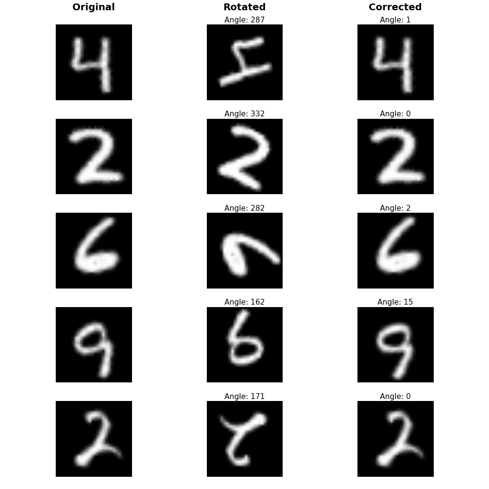
You can generate more of these examples by yourself using the display_examples function as shown in this Jupyter notebook.
Note that this model can be trained using a CPU as it doesn’t have much complexity. In practice, neural networks with many layers are always trained using parallel processing on GPUs.
RotNet on Google Street View
The MNIST dataset is a good choice for training your models if you want to quickly prototype a new idea because the size of the images is small and their content is relatively simple. This means that you don’t have to use very complex networks with many layers that would take a very long time to train.
But now that we know that our approach works well with simple handwritten digits, why not try with real life images? The Google Street View dataset, containing 62,058 high-quality Google Street View images is a good option for this. Out of those, we only choose the side views without markers overlaid on them (more details about what this means in the link above), which leaves us with 41,372 images. We select 90% of those as training images and the remaining 10% as validation images.
Here I provide the functionality to download the dataset and load two lists with the paths of the train and test images. To use it simply run:
from data.street_view import get_filenames as get_street_view_filenames

data_path = ... # location where you want to save the data
train_filenames, test_filenames = get_street_view_filenames(data_path)
Note that in this case, we are not loading all the images into memory as we did on the MNIST example. If we did that, we would run out of memory because these images have a much higher resolution. Instead, we are going to modify the RotNetDataGenerator to allow loading, cropping and resizing images. Cropping is needed because the network will only accept square images and the images in the Google Street View dataset are rectangular. We need to crop the centre of the image (or the right-hand side) because all the images have an overlaid icon on the upper-left side and we don’t want the network to only look for the position of that icon in order to predict the rotation angle. Resizing is needed to adapt the images to the input shape needed by the network. We also need to crop the image after rotation as described here. This is because if we left out the black borders, the network could simply figure out the rotation angle based on that. Moreover, it’s important to rotate the images before resizing them to avoid having interpolation artefacts at low resolutions (since we can’t binarize them as we did with the MNIST samples).
All of these operations can be achieved by replacing the rotate function in RotNetDataGenerator by the following generate_rotated_image function:
def generate_rotated_image(image, angle, size=None, crop_center=False,
                           crop_largest_rect=False):
    height, width = image.shape[:2]
    if crop_center:
        if width < height:
            height = width
        else:
            width = height
        image = crop_around_center(image, height, width)

    image = rotate(image, angle)

    if crop_largest_rect:
        image = crop_largest_rectangle(image, angle, height, width)

    if size:
        image = cv2.resize(image, size)

    return image
Here you can see the full implementation of the RotNetDataGenerator that also accepts image file paths as input. If you run the code by yourself you might find that the generator is somewhat slow. This is because loading high-resolution images and applying all the preprocessing operations on-the-fly is a costly operation. An alternative option would be to preprocess all the images and save them to disk, for example by generating 359 rotated versions out of each single image. For the sake of brevity, I have decided to keep using the generator approach.
Since the data in this example is more complicated, we will use a CNN architecture with more layers. In particular, we will use a deep residual network with 50 layers known as ResNet50. Keras already comes with a script to define this model, so we don’t have to do it ourselves. Even if you don’t know what the residual part means, we can train this network in a similar way as we did in the MNIST example. Keras also offers the possibility of loading this network with a model pre-trained on ImageNet data (ImageNet is a popular dataset containing 1.2 million images of 1,000 different classes typically used to train object recognition models). Starting the training process with pre-trained weights is usually faster than starting from random weights because we only need to slightly modify them. This is because models pre-trained for other computer vision tasks contain weights that are highly transferable, so we only need to fine-tune them. Moreover, complex models such as ResNet50 need a lot of data to be trained from scratch. Model fine-tuning can be typically done using much fewer data provided that the model was pre-trained using a large enough dataset containing samples similar to ours.
We can load the pre-trained ResNet50 model as follows:
# input image shape
input_shape = (224, 224, 3)

# load base model
base_model = ResNet50(weights='imagenet', include_top=False,
                      input_shape=input_shape)
In order to adapt the model to our application, we need to append a fully-connected layer at the end to generate the vector containing the 360 class probabilities:
# number of classes
nb_classes = 360

# append classification layer
x = base_model.output
x = Flatten()(x)
final_output = Dense(nb_classes, activation='softmax', name='fc360')(x)

# create the new model
model = Model(input=base_model.input, output=final_output)
Now we are ready to compile and train the model. These two steps are almost identical to the MNIST example. We just need to pass the appropriate parameters to the RotNetDataGenerator:
# model compilation
model.compile(loss='categorical_crossentropy',
              optimizer='adam',
              metrics=[angle_error])

# training parameters
batch_size = 64
nb_epoch = 50

# callbacks
checkpointer = ModelCheckpoint(
    filepath=output_filename,
    save_best_only=True
)
early_stopping = EarlyStopping(patience=2)
tensorboard = TensorBoard()

# training loop
model.fit_generator(
    RotNetDataGenerator(
        train_filenames,
        input_shape=input_shape,
        batch_size=batch_size,
        preprocess_func=preprocess_input,
        crop_center=True,
        crop_largest_rect=True,
        shuffle=True
    ),
    samples_per_epoch=len(train_filenames),
    nb_epoch=nb_epoch,
    validation_data=RotNetDataGenerator(
        test_filenames,
        input_shape=input_shape,
        batch_size=batch_size,
        preprocess_func=preprocess_input,
        crop_center=True,
        crop_largest_rect=True
    ),
    nb_val_samples=len(test_filenames),
    callbacks=[checkpointer, early_stopping, tensorboard]
)
Note that we are passing the preprocess_input function as a parameter to the generator. This function is used in Keras models that have been trained on ImageNet to normalise the input images before feeding them into the network.
Thanks to the use of pre-trained weights, we only need to wait for 10 epochs to get an average angle error of 1-2 degrees! Let’s look at some examples:
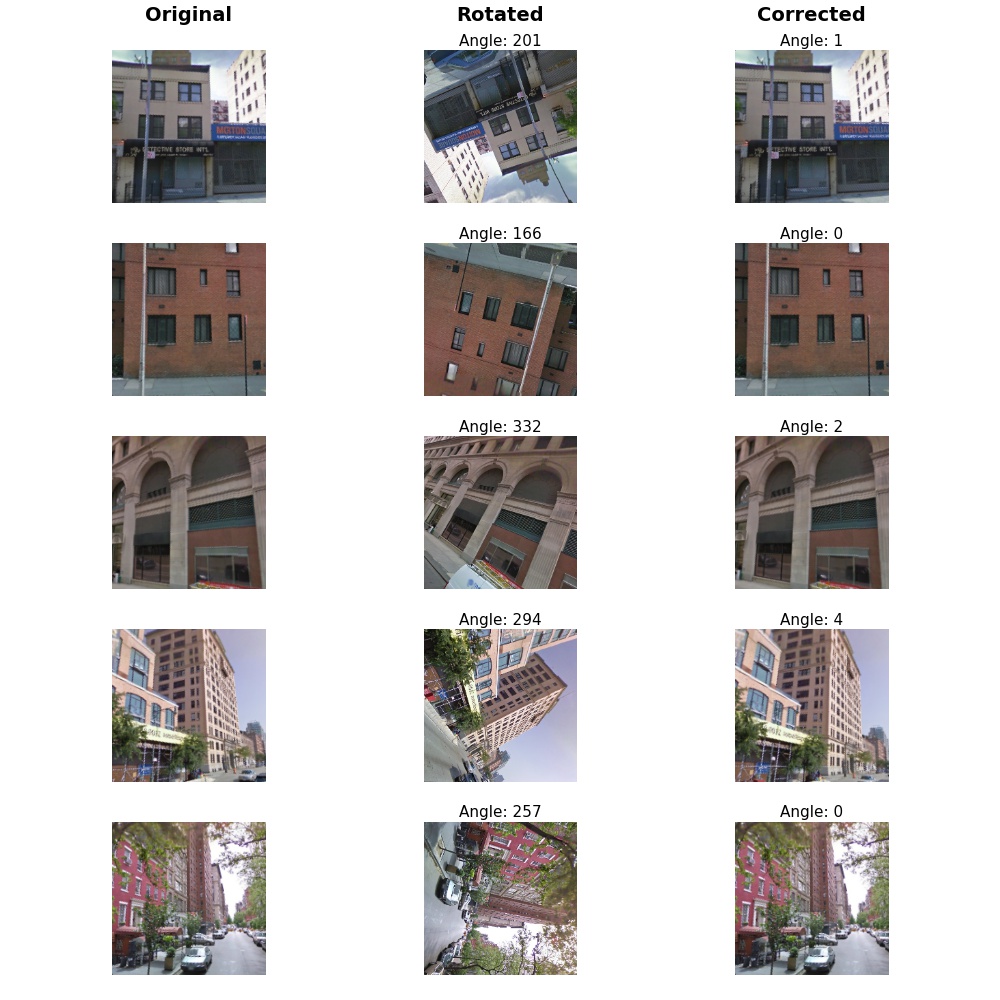
In the examples above, you can see that even when there is no sky or road, the network is able to correctly predict the rotation angle. You can generate more examples like these using this Jupyter notebook
One final note. It is unlikely that this model will perform well on images that are too different to our training images, so don’t expect it to work on images of objects and such. In order to make a model that generalises well to any image, we would need to find a dataset that contains more types of images and just train again (probably for a longer time). I will probably do this at some point, so keep an eye on the GitHub repository if you are interested!
Conclusions
We have seen how to train a convolutional neural network with data generated on-the-fly for the task of predicting the rotation angle of an image using Keras. With a minimum knowledge of neural networks, it is easy to train our own models by using commonly used architectures. As you might have noticed, obtaining and preparing the data can, in many cases, be more challenging than defining and training the network itself.
Hopefully, this post will help you think about your own novel applications of neural networks. For people starting in the field, I hope the tutorial has been simple enough to follow and that you have seen how easy it can be to use deep learning algorithms. I encourage you to keep learning more about neural networks and, as you do that, you will discover more of their possibilities and awesomeness!
Finally, here are some online resources that have been invaluable for my own learning:
- Machine Learning - Stanford (Coursera): general machine learning course covering the most important concepts and algorithms. Great course for a machine learning beginner. If you need help with the solutions, I uploaded mine to my GitHub page here.
- CS231n: Convolutional Neural Networks for Visual Recognition - Stanford: in my opinion the best course on convolutional neural networks. It is focused on computer vision but it covers everything you need to know about deep learning. The video lectures (which you can find on YouTube) are great, so make sure you check them out. I have also uploaded the solutions for all the assignments of this course to my GitHub here. Andrej Karpathy’s blog (one of the instructors of the course) is also a great resource.
- Deep Learning book by Ian Goodfellow, Yoshua Bengio and Aaron Courville: written by three experts in the field, this book could be considered the bible of deep learning. Consider checking this out if you want to do deep learning research.